Reading time: 4 min 44 sec

Note: This post is intended for educational purpose. It gives you some insights and details regarding the topic. The contents are structured to enable you to do this DIY project by yourself!

These days, it’s pretty much straight forward to simulate physical systems in a computer. Running those governing equations in any high-level languages such as Python, Visual Basic, Java, etc., make our life easier. Visualization of complex concepts of mainstream subjects is easier than ever before. Thanks to the growing community of coders!

But it is far more interesting when these computer codes interact with real physical systems which we can be touched and smelled! This opens up unlimited opportunities to probe and understand the complexities of a physical system easily. Successful communication between computers and physical systems is usually ensured by some external interfacing device which bridges the data processing between a computer and a physical system. This interface is capable of controlling and interpreting the signals to and from the computer. Though it was hard to implement such devices before, recent advanced technologies combined with novel inventions enable us to do successful interfacing effortlessly. Let’s begin!

Here we discuss a realtime demonstration of phase-space plot and timeseries of a physical simple pendulum. We employ an interfacing technique between Simulink (the coding part) and a Simple Pendulum (the physical system of interest) using a popular microcontroller called Arduino. Simulink provides a friendly graphical editor that can be integrated with powerful algorithms of Matlab to simulate various complex systems. As the library blocks of Simulink are rich and customizable, complex tasks can be performed neatly and intuitively.

So here is our outline of your DIY project:

1. Install Arduino libraries for Simulink. (This enables Simulink to effectively communicate with Arduino)
2. Connect Arduino to computer using a USB cable.
3. Then connect the Arduino to a potentiometer which in turn is attached to the pendulum. (Enables Arduino to read varying voltage signals during oscillations)
4. Finally, logically set up various blocks in Simulink to probe the swings of the pendulum. Done!

The working model of pendulum looks like this (sorry for the cluttered wiring):

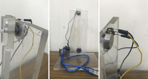
Here the pendulum oscillations are converted into corresponding voltage values using the potentiometer (pot). These values are read by Simulink through the Arduino Uno ADC, for further operations.

Selecting a proper pot: Here, the pendulum is attached to a potentiometer (10 Kohms, 1 rotation) which is powered by a 5V DC from Arduino and appropriately grounded. While oscillating, a variable voltage is passed to the analogue input of Arduino (pin: A0). Note that, not any pot can be used. The goal is to generate a maximum voltage difference between the endpoints of a half oscillation (I am confining my pendulum within 180-degree rotation). In our selected pot, 5 Kohms of resistance difference can generate a voltage difference of 5 Kohms/10 Kohms x 5V = 2.5 V (i.e., if the microcontroller is capable of reading the voltage with a resolution of, let’s say, 0.01 V, then our angle resolution is 180 degrees x 0.01 V/2.5 V = 0.72 degree). Though a 100 Kohms pot (with 10 rotations) can generate a same amount of resistance difference (5 Kohms), it can only generate a voltage difference of (5 Kohms/100 Kohms) x 5V = 0.25 V. So a minimum number of rotations with maximum DC voltage is preferred for better signal resolution. The total resistance value of the pot has no significance. (Alternatively, you may even go for an encoder for better resolution.)

Datatype and sampling rate: Once the libraries of Arduino are installed in Simulink, it is time to understand about the datatype and sampling rate of the signal from the Arduino. There is a dedicated block for capturing Arduino analogue input. Just drag and drop it from Simulink library. The output of this block is of datatype uint16. Since this type of data can’t always be compatible with the operations inside our remaining blocks, we include a data conversion block, to convert the datatype from unit16 to double. Regarding the sampling rate, Arduino (a 10 bit ADC) chops the analogue voltage reference into 1024 (2^10) steps. This simply means that Arduino can read the voltage values from 0 to 5V (Our reference voltage) in 1024 steps. So the voltage resolution is 5 V/ (1024-1) = 4.887 mV and the sampling rate is 204 voltage-samples per second. Arduino can send 204 voltage values to the computer every second (ExpEyes has a better resolution as it is a 12-bit microcontroller). Note that the Arduino analogue block has a handle to override the sampling rate manually. (I have set to 100 samples ps, in our case; green color lines in the below block diagram)

The Simulink block diagram is given below:

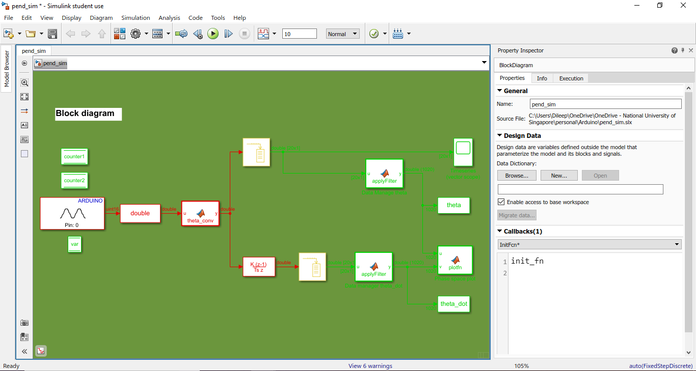
Angle calibration block (Block name: theta_conv): This is just to convert your voltage values to corresponding angular values in radians. A ‘Matlab Function block’ is used for signal-scaling with a proper mathematical equation.

After the theta_conv block, the signal diverts into two branches to process the signals for filtering and differentiation. You may call the upper branch as ‘theta branch’ and lower branch as ‘theta-derivative’ branch. A discrete derivative block is placed first in the lower branch, which takes the derivative of theta input.

The trade-off between noise reduction and sampling rate: To reduce the fluctuations in the voltage signal, a Savitzky–Golay filter can be used effectively inside a Matlab Function block (‘applyFilter’ in the block diagram). But for a filter to work properly, it is advisable to use a buffer to pick and store ~20 voltage signal data. But then the buffer has to wait for 20 signals to arrive, thereby compromising the sampling rate of all the following blocks. Greater the buffer value, better the noise reduction, and poorer the sampling rate. In our case, the buffer value is 20 (0.01 sec x 20 = 0.2 sec to collect the data and give it to the output), and this results in a sampling rate of 5 samples ps. The sampling rate of the rest of our calculations is now 0.2 sec (green color lines in the block diagram). In a realtime plotting scenario, like ours, the sampling rate of the plotting signal matters. So wisely choose the buffer value.

Plotting function and initialization code: Once the theta and theta derivatives (in sets of 20 data per sec) are available, it is time to plot them. It’s a good idea to initialise a Matlab figure with proper handles before running the code. You may save your initialization script (let’s say, ‘init.m’) in the Simulink file folder, and add the script-name to the ‘InitFcn’ of your ‘callbacks’ of the Simulink. You may also add an oscilloscope block in the theta branch to see the time series of the oscillations.

OK, let’s see the working model:

Additional notes:

1. Check always that the sampling rate of every block is proper. It is a good habit to inherit (-1 value) the rate from the previous block.
2. Defining variables: You need to define variable-size arrays during coding. I prefer to go for the ‘persistent’ command to do so. It is neat and comfortable.
3. The counters in the block diagram are data memory blocks which intelligently keep track of the sampling rate after data buffering. The variable (datatype: double) set inside these blocks are global variables so that they are callable within functions. These blocks mimic loops in ordinary code.
4. Angle calibration has to be done physically before feeding the calibrated data to theta_conv block.
5. You may add additional blocks ‘To Workspace’ for the post processing of your data.

Happy coding!