Reading time: 5 min 10 sec, Machine Learning skill required: Intermediate

But why should you be bothered about predicting the academic success of a student? Early detection of students at the risk of failure can substantially boost their success probability when sufficient measures are taken from the teachers’ side. With the recent advent of computational power, lengthy and sophisticated numerical calculations can now be carried out in seconds!

A note on the data used in this article: Efficient data mining can provide useful input-features for ML to predict accurate outcomes. Any supervised ML technique needs a large amount of useful data as input. This data is cleverly visualized for manually eliminating the redundant features and gaining other insights. Based on these insights, the data is further pre-processed (such as normalization, weightage-implementation and others) and fed into the ML algorithm. Careful and systematic implementation of such a pre-processed data in ML can significantly cut-down the computational cost and time required for your calculations. There are several techniques widely used to choose the right amount of data with significant features.

Problem definition: We have collected the examination marks of 1000 students (for their half-yearly examination) who had differently scored in three subjects, Maths, Physics and Chemistry. Also, we have the data on these students’ success (or failure) in their final-year examination. Our task is to find out a pattern connecting a student’s performance in his half-yearly examinations and his success in the final-year examination. Once an optimized pattern is available, we can predict a fresh student’s success (or failure) in his final-year examination based on the marks he scored in the half-yearly examination.

In our case, for simplicity, we have taken only three features (marks in three subjects) to predict whether a student passes the final examination or not (the data is taken from Kaggle.com). The code in this article is written in python 3.7.4 (IDE: spyder). At first, let’s have a look at the data in hand:

In [1]: # -*- coding: utf-8 -*-
"""
Created on Tue Jun 23 21:53:10 2020
@author: Dileep Kottilil
"""
import pandas as pd
from pandas.plotting import scatter_matrix
import numpy as np
import matplotlib.pyplot as plt
from sklearn.model_selection import train_test_split
from sklearn.linear_model import LogisticRegression
from sklearn.metrics import accuracy_score
from sklearn.metrics import confusion_matrix
from sklearn.metrics import classification_report
from sklearn.model_selection import validation_curve
from mlxtend.plotting import plot_learning_curves 
from mlxtend.plotting import plot_decision_regions

# Sampling of data
#--------------------------------------------------------#
data = pd.read_csv("Student_dataset.csv")
data.head()

Out [1]:
   Maths  Physics  Chemistry  Result
0     17       27         22       0
1     72       82         77       1
2     97       18         13       0
3      8       42         37       0
4     32       25         20       0

Here, many packages are initially imported into the python workspace for the complete ML calculations. The output shows the first 5 rows of the data collected. Each row corresponds to the performance of a student. The output has four columns where the first three columns represent input features (Marks obtained for Maths, Physics, Chemistry), and the fourth one is called the target (Result). The value of Result ‘1’ (‘0’) indicates the success (failure) of that particular student in the final examination. Our task, as stated previously, is to recognize a relationship between these input features and the target.

Data visualization: A histogram and a scatter-plot can be plotted for the three features to get an initial insight into the given data.

# Splitting features and target into two matrices X and y
X = data.drop("Result",axis = 1)
y = data.Result

# histogram plotting
histax = X.hist()
for ax in histax.flatten():
    ax.set_xlabel("Marks")
    ax.set_ylabel("Number of students")
plt.tight_layout()
plt.show()

# Check for the correlations between features
plt.figure(1)
scatter_matrix(data.iloc[:,0:3])
plt.show()

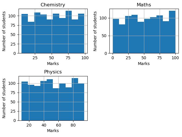
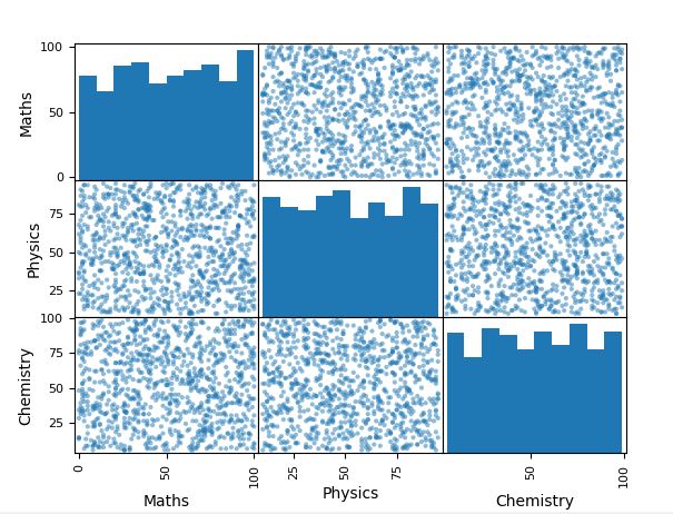
The histogram and scatter plot of the features are shown above. If you look at the scatter plot, you may notice a random distribution of data-points in the off-diagonal plots. This indicates no correlation between the features. Any type of correlation can be easily identified if you obtain any pattern for off-diagonal plots.

The algorithm: We will use one of the best and simplest algorithms widely used by the ML community from all around the world: Logistic Regression. Although the algorithm is linear, its versatile nature to implement in many complex data structures makes it unique and reliable. As a first step, we will try to find out whether this algorithm requires regularization or not. Regularization is a process of effective management of the weights assigned to the features. The regularised parameter value (this controls the regularization process), often called lambda, tunes the model into an optimized form, free from both underfitting and overfitting. The choice of lambda is based on the performance score calculated based on the cross-validation set (Yes! I am introducing new words without defining it. Please refer to the basics if your ML skill level is less than intermediate). The following code shows the optimized lambda value by plotting the validation curve.

# selection of optmized lambda value from validation curve
#--------------------------------------------------------#

# Data splitting into train and test data
X_train, X_test, Y_train, Y_test = train_test_split(X, y, test_size=0.20, 
                                                    random_state=1)

lambda_val = np.linspace(0.1,100,num = 50)

# Selection of algorithm
model = LogisticRegression(solver='liblinear')

# Sweeping the regularization parameter, lambda.
train_scores, test_scores = validation_curve(model, X_train, Y_train, 
                                             param_name="C", 
                                             param_range=1/lambda_val,
                                             scoring="accuracy", n_jobs=1)
train_scores_mean = np.mean(train_scores, axis=1)
train_scores_std = np.std(train_scores, axis=1)
test_scores_mean = np.mean(test_scores, axis=1)
test_scores_std = np.std(test_scores, axis=1)

# plotting validation curve
plt.figure(3)
plt.title("Validation Curve with LR")
plt.xlabel("lambda")
plt.ylabel("Score")
plt.ylim(0.75, 0.9)
lw = 2

plt.plot(lambda_val, train_scores_mean, label="Training score",
              color="darkorange", lw=lw)
plt.fill_between(lambda_val, train_scores_mean - train_scores_std,
                  train_scores_mean + train_scores_std, alpha=0.2,
                  color="darkorange", lw=lw)
plt.plot(lambda_val, test_scores_mean, label="Cross-validation score",
              color="navy", lw=lw)
plt.fill_between(lambda_val, test_scores_mean - test_scores_std,
                  test_scores_mean + test_scores_std, alpha=0.2,
                  color="navy", lw=lw)
plt.legend(loc="best")
plt.show()

The accuracy score decreases after lambda = 2 and finally becomes a constant for both the training set and cross-validation dataset (Please refer to the above code to understand how the main dataset is split into training and cross-validation sets). As the accuracy score is highest for lambda = 2, we fix this lambda for our actual modelling below. Before that, we need to check the influence of the number of data points on the prediction outcome. This is important in case if ‘1000’ data points are not enough for accurate predictions. So, we plot the learning curve as below:

# Plot of learning curve
#--------------------------------------------------------#

# Final model is decided after selecting optimized lambda value
model_final = LogisticRegression(solver='liblinear',C = 1/2)

# Splitting train data into train and cross validation data to obtain learning curve
X_train1, X_cv = X_train[:len(X)], X_train[:len(y)] 
Y_train1, Y_cv = Y_train[:len(X)], Y_train[:len(y)] 

plt.figure(4).tight_layout()
plot_learning_curves(X_train1,Y_train1,X_cv,Y_cv,model_final,scoring = 'accuracy')
plt.show()

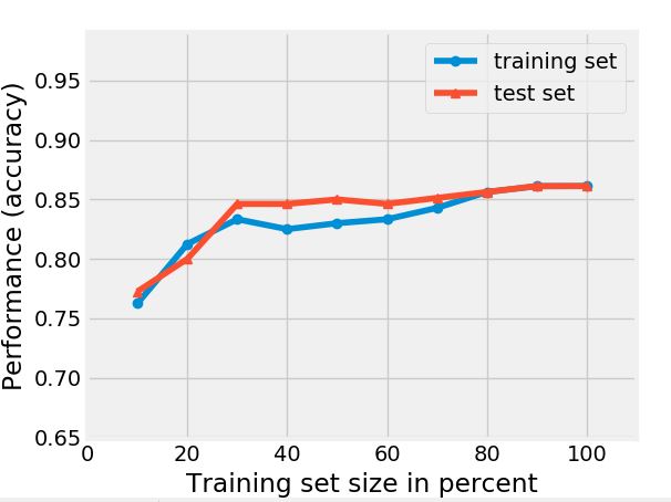
The learning curve shows that the prediction accuracy score is the same for both test and training data after 800 (80% of the total data) data entries. This indicates that to predict an outcome with 85% accuracy (y-axis), you only need 800 data points. Since we already have 1000 data points, we can safely say that we have sufficient data.

A note on the performance score: It’s possible to increase the performance score by adding more influencing features such as the student’s age, family background, economic status, health conditions and many more. In addition to that, the number of data entries is a crucial factor that determines the performance of an algorithm. Learning curves help you get an idea about the number of data points needed for your algorithms’ excellent performance.

Finally, we plot the decision boundaries showing both the data entries and the feature space’s prediction regions. These plots help us understand whether the model can contain the ‘target’ classes (‘0’ and ‘1’) within the predicted class boundaries.

Let’s look at the first plot in the above grid-plot. The blue (red) region corresponds to the predicted failed (success) region. Blue (red) data points are our input data. If blue (red) data points come inside the blue (red) region, then we can safely say that our algorithm works well in predicting the success and failure of a student. In this case, the decision boundary is the line separating the blue and red region. Each plot in the grid indicates different decision boundaries when a student’s mark obtained in Chemistry is different. Okay, let’s interpret it: For example, consider our last plot (lowermost-right) in the grid. This plot is applicable for a student if he scores 80 +/- 5 (refer to the code) marks in Chemistry. Such a student has a higher chance of success if his marks in Maths and Chemistry lie in the red region. In the same way, every plot in the grid can be visually interpreted. Of course, our prediction is not 100% accurate as some data points are not lying in the correct regions.

Finally, let’s predict the performance of this algorithm on an unseen data:

# predicting the performance metrics by applying the model on the test (unseen) data
#--------------------------------------------------------#

model_final.fit(X_train, Y_train)
predictions = model_final.predict(X_test)
print("accuracy score for LR model is",accuracy_score(Y_test, predictions))
print(classification_report(Y_test, predictions))

Output:
accuracy score for LR model is 0.875
              precision    recall  f1-score   support

           0       0.88      0.97      0.92       154
           1       0.84      0.57      0.68        46

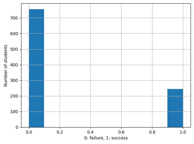
The output shown above reveals that the accuracy of our model is 87.5 %. More importantly, there is another excellent performance metric called f1 score (a value between 0 and 1), which is more reliable than the accuracy score. Our most important aim in an ML prediction task is to increase the f1 score to 1. In our case, the f1 score is 0.92 for predicting the failure and 0.62 for predicting the success. One reason for the poor f1 score for predicting success is our skewed data itself. If you look at the histogram below, more failure data is available compared to the success data.

Therefore, our model is not as accurate as possible. To overcome this issue, there are many tricks. One straightforward way is to delete some ‘failure data’ from our data set to create an unbiased dataset. Below is the prediction results after eliminating 67% of the failure data points from our primary dataset (of course, deleting data points will affect, validation and learning curves. But just ignore that for a moment).

accuracy score for LR model is 0.8080808080808081
              precision    recall  f1-score   support

           0       0.79      0.77      0.78        43
           1       0.82      0.84      0.83        56

Now f1 score for the ‘failure data’ has improved, but still not the best. As I said before, it is possible to play around with this code to enhance its performance.

I Hope, you have gained a few insights about how to implement a supervised ML Linear Regression algorithm to predict your success in the final examination! If you liked this article, please do subscribe, share and hit the like button.

For more details, contact me. Happy coding!