Reading time ~5 min

Have you ever witnessed the learning process of a Machine Learning (ML) algorithm? Today, you are going to see how an ML algorithm learns and creates its own model from the given data. As an example, let’s consider a linear data set where the ‘y’ values are a linear function of ‘x’ values. You might have done such linear curve fitting tasks ‘n’ number of times (where n tends to a large value!) in your life using popular software such as Matlab, Mathematica or Origin. But have you ever wondered what’s happening behind the scenes? Have you ever seen the iterative process of refining a model step by step in real-time? If not, this article is for you because it’s quite interesting to watch such a process. In this article, you are going to see how data modelling (curve fitting) can be done using an ML algorithm. As I said before, since the data in our hand shows some linear dependence, we are going to model this data using a Linear Regression (LR) algorithm called gradient descent.

Background: Linear regression is a method of finding a linear relationship between the response (‘y’) and variables (‘X’). And, gradient descent is just one of the many algorithms used in ML (or in any fitting software) to find out the best linear model. Here, our job is to formulate a convex function (sometimes called cost function with variables ‘slope’ and ‘y-intercept’) whose minimum value corresponds to the best linear model. The gradient descent algorithm minimizes this cost function at each iteration under the right conditions. In this context, such a minimization process is called convergence. If you are interested in the underlying math, you may click here for details.

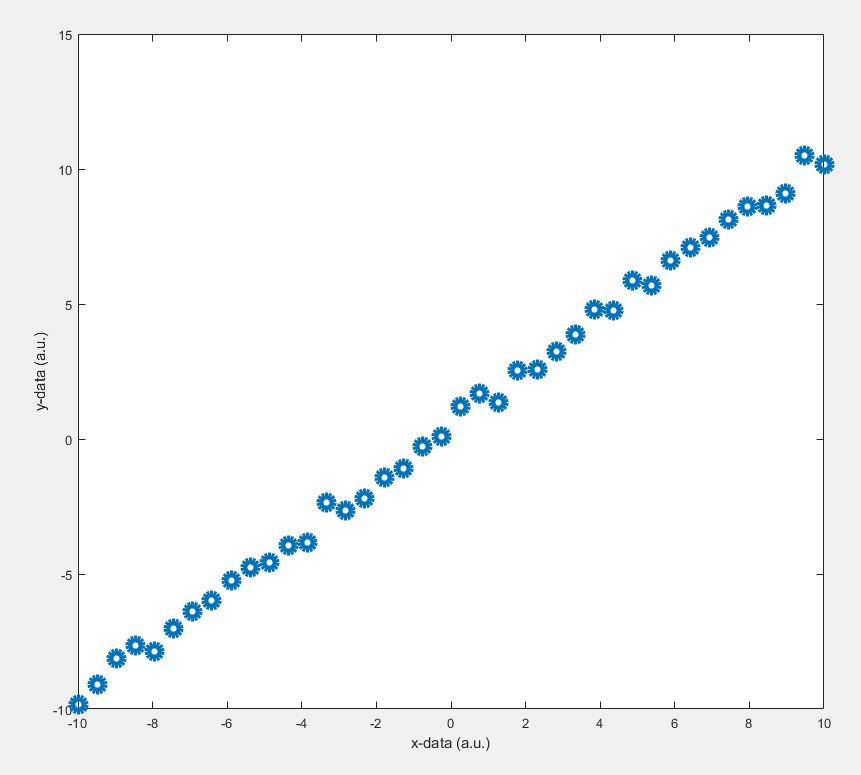
In the gradient descent algorithm, there is a tuning parameter called ‘learning rate’ that decides the behaviour of the algorithm itself. Depending on the value of the ‘learning rate’, the algorithm may or may not converge into the best model. It also decides the time required for the convergence. The gradient descent algorithm moves towards the best model, while the ‘learning rate’ determines the step size between the two consecutive models. Depending on this value, the model can be oscillatory, convergent or divergent. We will see all that in a moment. At first, let’s have a look at the data to be fitted.

The value of ‘learning rate’ is a key factor for your algorithm to converge

Coding: Okay. As I promised in the title, now we going to see how this algorithm finds the best model through iterative steps. Let’s dive into the complete code (The code is written in Octave 5.2. You may run it in Matlab as well):

clear; clc;
y = linspace(-10,10,40)'+rand(1,40)'; % y data
m = length(y); % number of training examples
X = [ones(m, 1), linspace(-10,10,40)']; % x data

% initialize fitting parameters
theta = [-0.05;-2]; % 1st and 2nd values correspond to y-intercept and slope respectively
num_iter = 50; % number of iterations
alpha = 0.01; %learning rate 

%initializing zero matrices
theta_mat = zeros(2,num_iter);
J_mat = zeros(1,num_iter);
thr = 0.01; % convergence threhsold

%initializing a figure
figure
set(gcf, 'Units', 'Normalized', 'OuterPosition', [0, 0.04, 1, 0.96]);

% optimizing parameters slope and y-intercept
for iter = 1:num_iter 
	theta_old = theta;
    predict = X*theta_old;
	theta(1,1) = theta_old(1,1)-(alpha/m*sum(((predict-y).*X(:,1)))); % updating y-intercept values
	theta(2,1) = theta_old(2,1)-(alpha/m*sum(((predict-y).*X(:,2)))); % updating slope values
    J = (1/(2*m))*sum(((predict)-y).^2); % cost function
    
	theta_mat(:,iter) = theta; % creating theta matrix
    J_mat(1,iter) = J;         % creating cost function matrix
	disp(iter)
	p(1) = subplot(2,3,[1,4]);plot(X(:,2), y, 'o','MarkerSize',15,'LineWidth',5)
	xlabel('x-data (a.u.)')
    ylabel('y-data (a.u.)')
    hold on
	plot(X(:,2), predict, '-','LineWidth',8)
    ylim([-20,20])
    hold off
	title('Fitted plot')
	legend(p(1),'Data', 'Model')

	p(2) = subplot(2,3,[2]); plot(1:iter,theta_mat(1,1:iter),'-or','MarkerSize',10,'LineWidth',4)
	title('predicted values of y-intercept')
	xlabel('no. of iterations')
    ylabel('y-intercept (a.u.)')
    
	p(3) = subplot(2,3,[5]); plot(1:iter,theta_mat(2,1:iter),'-ob','MarkerSize',10,'LineWidth',4)
	title('predicted values of slope')
    xlabel('no. of iterations')
    ylabel('slope (a.u)')
    
	p(4) = subplot(2,3,[3,6]); plot(1:iter,J_mat(1:iter),'-o','MarkerSize',10,'LineWidth',4)
	title('Cost function')
    xlim([p(4),p(2),p(3)],[0,num_iter])
    xlabel('no. of iterations')
    ylabel('Cost function)')
  	pause(0.01)

    % searching for convergence condition
	if abs(theta(2,1)-theta_old(2,1))<0.01 && abs(theta(1,1)-theta_old(1,1)) < thr
		break;
	end	
end
disp('The end')

By setting the learning rate as 0.01, you can see the convergence of the slope value, thereby the model, after a few iterations. Iterations will stop when the convergence threshold is met. You can see how bad the initial model is (orange line in the leftmost figure). But gradually this initial model refines itself over many iterations and eventually takes the form of the best fit. This is the learning process we are talking about.

Note that convergence will only happen if the cost function gradually drops as evident from the rightmost figure. Now, changing the learning rate to 0.06, you can see a diverging model. The slope is shooting up in an oscillatory fashion after each iteration, and the corresponding fitted line is moving away from the actual data points.

Considering the third case, by setting the learning rate as 0.05, the model undergoes a damped oscillatory path (see the figure below) towards the convergence point. You can see that the initial model oscillates around the data points with a declining amplitude. The cost function gradually converges (rightmost figure) and eventually settles at the minimum.

Now, let’s see a pure oscillatory behaviour; neither convergent nor divergent. Such models oscillate indefinitely around the original data. By setting a magic value, 0.0571211` as the ‘learning rate’, you can see an oscillatory behaviour. In this case, the cost function takes a linear response.

Okay, now it’s clear that choosing the right value for the ‘learning rate’ has a significant role in the way an algorithm behaves. You have just witnessed it. User-friendly software such as Python, Matlab or Mathematica, do this job very nicely without getting you involved. However, it is always better to get involved and have a sense of what is happening behind-the-scenes so that you can design and tune your own algorithms for your complex models.

By the way, from this article, do you think that ML is nothing but an ‘honoured’ curve fitting? 😛 Comment your thoughts below.

If you like this article please rate and share.