Reading time: 4 min 2 sec

Can machines learn just like humans do? If that is possible, will that be a threat to humanity? You might have seen apocalypse-themed movies and shows such as Terminator series or Westworld wherein intelligent machines become sentient and eventually turn against humans. Will such scenarios ever become a reality in the future? No one knows for sure. Whether such an outcome is inexorable or not, what you have to understand is that machines can learn just like humans do! Don’t worry, if we train them in the right manner, we can make this world a better place. In simple terms, such a process of training the machines to learn and predict events or patterns autonomously based on available data is called Machine Learning (ML). ML can be applied to predict the weather, stock market fluctuations, evolutionary mutations and many more. As an example, today, we are going to focus on predicting the chance of a heart attack in a patient. Accurate prediction of heart attacks can aid timely treatment saving millions of lives.

Although a heart attack happens because of pure biological reasons, it is quite possible to predict it without knowing anything about biology! Using the data associated with parameters such as blood pressure, severity of chest pain, blood sugar level and many others, ML can predict the chance of a heart attack. Now, are you interested to learn ML? In this tutorial, we are going to learn how to predict a possible heart attack using several ML algorithms. Then, we will select the best algorithm that makes the most accurate predictions and find a relation between the anomalies in the body parameters and the chance of a heart attack.

Although this tutorial is not primarily meant for covering all the basics of ML, we will quickly go through the essentials of a specific class of ML called supervised ML. Being a part of artificial intelligence (AI), supervised ML looks for patterns in a massive labelled data given. Patterns (these are nothing but complex mathematical equations to fit the data) are recognized with the help of algorithms we input. Once a pattern is identified, the machine can make predictions on new unused data based on the identified patterns. Unlike conventional procedural programming, ML doesn’t require any initial guesses or models to generate a governing pattern. It does everything autonomously. Impressive, isn’t it?

Our goal: We have a large excel sheet containing many patients’ data taken from the repository of Kangle. A glimpse of data is given:

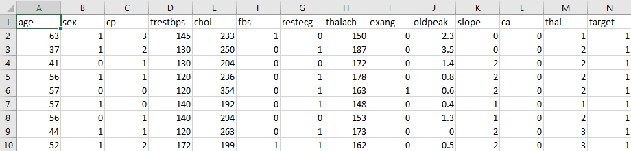
Every column represents a parameter such as ‘age’, ‘sex’, ‘cp’ (chest pain) and others (The description of all the columns is out of the scope of this tutorial). Some data entries are boolean (0 or 1 only), representing the presence (true) or absence (false) of a particular parameter. For instance, a 0 value of ‘cp’ indicates the absence of chest pain. As another example, 0 in ‘restecg’ represents the normal value of rest ECG. The final column ‘target’ (or N) indicates whether that patient experienced a heart attack (1) or not (0). In this data, we can consider columns A to M as influencing parameters for a heart attack. Our goal is to find out a pattern (model) between these parameters, that results in a heart attack (1 in ‘target’) or not (0 in ‘target’). So, our task can be called as a classification problem in ML.

Language: We are going to use Python 3.7.6 (IDE: spyder 4.0.1) as the coding language to achieve our goal. Now, let’s have a look at the general flow-chart of the supervised ML process.

Flowchart: A massive raw data representative of the general trend of a phenomenon is labelled and preprocessed (such as scaling and normalization). The resultant data is split into training data (70%) and testing data (30%). This proportion can be varied. Then a set of linear and nonlinear algorithms are used to test the prediction accuracy of the algorithm in the training data (which will further split into 70 and 30% during the process of finding the pattern). Once an algorithm detects a model, it predicts the chance of a heart attack in a patient. The corresponding metric of prediction accuracy can be calculated.

Coding: Now, the fun part begins! In Python, you have to import three main libraries: sklearn, pandas and matplotlib. Sklearn contains the most effective tools to do predictive analytic techniques in ML. Pandas library is meant for fast, flexible and powerful data processing. Finally, matplotlib is a versatile library for data visualization. Let’s import all the necessary libraries in Python first:

import warnings
warnings.filterwarnings('always')  # import warnings on every run: "error", "ignore", "always", "default", "module" or "once"

import pandas as pd
from matplotlib import pyplot
from sklearn.model_selection import train_test_split
from sklearn.model_selection import cross_val_score
from sklearn.model_selection import StratifiedKFold
from sklearn.metrics import accuracy_score
from sklearn.linear_model import LogisticRegression
from sklearn.neighbors import KNeighborsClassifier
from sklearn.svm import SVC
from sklearn import preprocessing

Once all the necessary libraries are imported, the next step is to import data file (.csv) from the device. Pandas library import data as a DataFrame object with which data processing is very flexible:

# Load dataset
filename = "C:/Users/heart.csv"
dataset = pd.read_csv(filename) #dataframe object

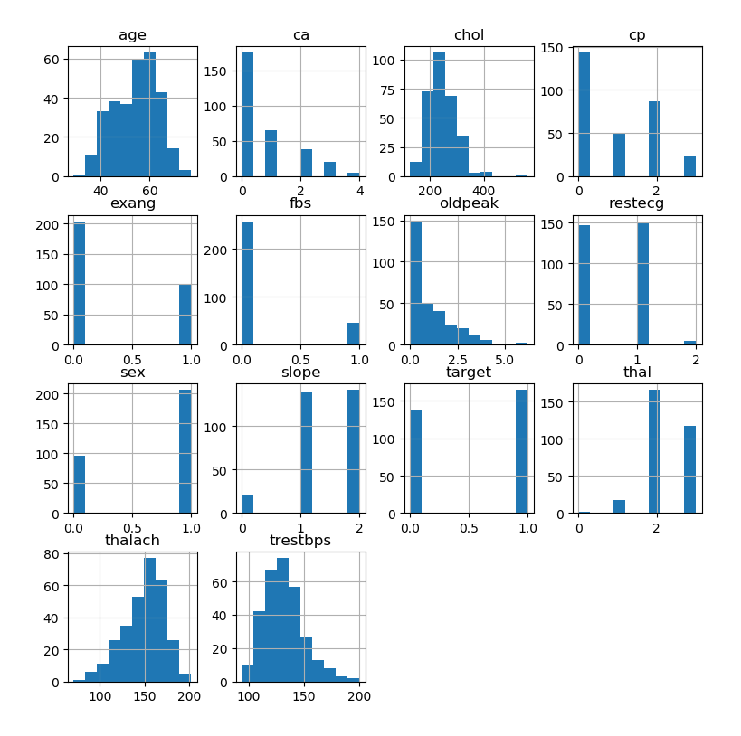
In order to get a visual feel of the raw data, let’s plot a histogram of these variables:

dataset.hist()
pyplot.show()

The histogram is shown below:

Then we scale (known as data preprocessing) a few columns using the StandardScalar() function so that all the columns are in the same scale. Failing to do so might have some effects in the final result:

#scale numerical data
standardScaler = preprocessing.StandardScaler()
columns_to_scale = ['age', 'trestbps', 'chol', 'thalach', 'oldpeak']
dataset[columns_to_scale] = standardScaler.fit_transform(dataset[columns_to_scale])

Next step is to split the raw data into two sets called variables (X, all columns except ‘target’) and response (y, column ‘target’). Here, the values of variables for each row collectively determine the binary state of the ‘target’ column.

Now, it’s time to split the data into training and testing data:

X = dataset.drop(['target'],axis=1)
y = dataset['target']
X_train, X_validation, Y_train, Y_validation = train_test_split(X, y, test_size=0.3,random_state=1)
#replace 0 to no_attack and 1 to attack. This has no effect in the algorithms to be used.
dataset['target'] = dataset['target'].replace([0,1],['no_attack','attack'])

Then we adopt three algorithms, LR (Logistic Regression), KNN (K-Neighbors Classifiers), SVM (Support Vector Clustering) to find and learn the hidden pattern connecting X and y. Within the ‘for’ loop, each algorithm is trained and tested with the training data, and eventually, the loop throws an accuracy metric. This metric is used to evaluate the performance score of each algorithm. The code is given below:

#Algorithms
models.append(('SVM', SVC(kernel='sigmoid',gamma='auto')))
models.append(('LR', LogisticRegression(solver='liblinear', multi_class='ovr')))
models.append(('KNN', KNeighborsClassifier(n_neighbors=8)))

# evaluate each model in turn
results = []
names = []
for name, model in models:
	kfold = StratifiedKFold(n_splits=10, random_state=1, shuffle=True) 
	cv_results = cross_val_score(model, X_train, Y_train, cv=kfold, scoring='accuracy')
	results.append(cv_results)
	names.append(name)
	print('%s: %f (%f)' % (name, cv_results.mean(), cv_results.std()))

Keep in mind that every algorithm generates its own model to predict the binary state of y from X. The performance of these models in predicting y is determined using a metric called “accuracy score”. When you run the program you get the accuracy score for each algorithm:

Here, both SVM and LR show almost the same accuracy. So we can try both algorithms to fit the testing data (30%) which we split initially. Corresponding accuracy scores are below:

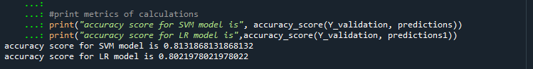
Here, the accuracy score of the SVM model is slightly greater than that of the LR. Therefore, in principle, we have to do further tune the parameters of algorithms to get the best among them. Anyway, for now, we can consider the SVM as the best one because it has better accuracy score (0.81) on the unseen data.

So, we have predicted the chance of a heart attack in a patient with 81.3% of accuracy with our machine learning SVM algorithm. Now, it’s a matter of feeding fresh data to this model to predict as many cases as possible. Happy coding!

Note: If you would like to receive the complete code and the raw data file, please subscribe to the blog, and just ping me through the Contact menu.